Wärmestrom

https://learnsql.com/blog/moving-average-in-sql/ https://stackoverflow.com/questions/55491046/how-to-set-the-running-file-path-of-jupyter-in-vscode

Get Wärmestrom data

By querying directly the SQLite table and filtering by meter id. But for Wärmestrom we have two different meters, because there are two tarifs depending on the time of the day.

%%sql 

CREATE OR REPLACE TABLE waermestrom_sqlite AS 
SELECT 
  meterid, 
  -- Blob Functions, because most columns get read as blob
  -- https://duckdb.org/docs/sql/functions/blob
  decode(date)::DATETIME AS date, 
  decode(value)::INT AS value
FROM sqlite_scan('{{latest_file}}', 'reading') 
WHERE meterid = 2 OR meterid = 3
;
SELECT * FROM waermestrom_sqlite;

	meterid	date	value
0	3	2020-11-30 17:36:00	9773
1	2	2020-11-30 17:36:00	9456
2	2	2020-12-01 00:00:00	9464
3	3	2020-12-01 00:00:00	9779
4	2	2020-12-01 14:23:00	9470
...	...	...	...
4728	3	2026-04-07 08:20:00	6035
4729	2	2026-04-11 23:42:00	5023
4730	3	2026-04-11 23:42:00	6052
4731	3	2026-04-12 09:12:00	6052
4732	2	2026-04-12 09:12:00	5027

4733 rows × 3 columns

Ideally, there would be one measurement for each tarif, for every date (minute). But we cannot guarantee that’s the case (e.g. measurement for one tarif can be at 13:08:59 and for the other at 13:09:00). So let’s see if that’s the case.

%%sql 

SELECT date, count(*) AS cnt
FROM waermestrom_sqlite
GROUP BY date
;

	date	cnt
0	2020-11-30 17:36:00	2
1	2020-12-01 07:18:00	1
2	2020-12-01 07:19:00	1
3	2020-12-01 20:22:00	1
4	2020-12-03 02:38:00	2
...	...	...
2589	2026-02-25 08:38:00	2
2590	2026-02-26 09:25:00	2
2591	2026-03-07 21:03:00	2
2592	2026-03-15 16:24:00	2
2593	2026-04-03 20:58:00	2

2594 rows × 2 columns

Yeap, there are some cases with cnt=1. More precisely, the below number of cases:

%%sql 

WITH ucnt AS (
  SELECT date, count(*) AS cnt
  FROM waermestrom_sqlite
  GROUP BY date
)
SELECT cnt, COUNT(*) FROM ucnt GROUP BY cnt
;

	cnt	count_star()
0	1	455
1	2	2139

Safest would be to just join the dates and make sure to fill in the gaps with the closest value. Let’s see

%%sql

CREATE OR REPLACE TABLE waermestrom_nulls AS
WITH
ws181 AS (
  SELECT 
    'Hoch' AS tariff,
    decode(date)::DATETIME AS date, 
    decode(value)::INT AS value
  FROM sqlite_scan('{{latest_file}}', 'reading') 
  WHERE meterid = 3 
),
ws182 AS (
  SELECT 
    'Niedrig' AS tariff, 
    decode(date)::DATETIME AS date, 
    decode(value)::INT AS value
  FROM sqlite_scan('{{latest_file}}', 'reading') 
  WHERE meterid = 2
)
SELECT
  COALESCE(ws181.date, ws182.date) AS date,
  ws181.value AS value_hoch,
  ws182.value AS value_niedrig
FROM ws181 
FULL JOIN ws182 
ON ws181.date = ws182.date
ORDER BY date
;
SELECT * FROM waermestrom_nulls LIMIT 20;

	date	value_hoch	value_niedrig
0	2016-07-04 07:50:00	0	0
1	2016-07-04 08:00:00	1	1
2	2016-11-28 00:21:00	547	<NA>
3	2016-11-28 15:23:00	<NA>	484
4	2017-11-25 15:20:00	3347	<NA>
5	2017-11-25 15:23:00	<NA>	2677
6	2018-11-23 15:19:00	5747	<NA>
7	2018-11-23 15:22:00	<NA>	4893
8	2019-11-29 14:18:00	7914	<NA>
9	2019-11-29 14:22:00	<NA>	7224
10	2020-11-30 07:07:00	9764	9456
11	2020-11-30 17:36:00	9773	9456
12	2020-12-01 00:00:00	9779	9464
13	2020-12-01 07:18:00	9782	<NA>
14	2020-12-01 07:19:00	<NA>	9470
15	2020-12-01 14:23:00	9792	9470
16	2020-12-01 20:21:00	9798	<NA>
17	2020-12-01 20:22:00	<NA>	9470
18	2020-12-02 00:01:00	9800	9473
19	2020-12-02 07:29:00	9802	9476

Yeah, those are the cases: 2020-12-01 07:18:00 has value hoch, but no niedrig 2020-12-01 07:19:00 has value niedrig, but no hoch

So now we want to fill in those gaps using the value of the same column, that has the closest date. So it’s tricky, because it cannot simply be a fill-down, or fill-up. Because in one case, the correct value would be one position up, and in other case one position down. Here’s one approach (it just assumes there are no consecutive nulls for the value columns; please also note that it takes advantage of DuckDB’s flexible SQL syntax -otherwhise it would have been even longer, with a bunch of CTEs-)

%%sql

CREATE OR REPLACE TABLE waermestrom_nonulls AS
SELECT
  date,
  value_hoch, value_niedrig, 
  -- calculate minutes diff with previous and next date, to see which is closer
  -- note the use of a default value for lag/lead, substracting and adding one day
  -- for lag and lead respectively, to avoid NULLs in the first and las rows
  date_sub('minute', lag(date, 1, date - INTERVAL 1 DAY) over(order by date), date) AS minutes_lag,
  date_sub('minute', date, lead(date, 1, date + INTERVAL 1 DAY) over(order by date)) AS minutes_lead,
  -- and we want to replace null values column, with the value from closest date
  CASE
    WHEN value_hoch IS NULL AND minutes_lag <= minutes_lead 
    THEN lag(value_hoch) over(order by date)
    WHEN value_hoch IS NULL AND minutes_lag > minutes_lead 
    THEN lead(value_hoch) over(order by date)
    ELSE value_hoch
  END AS value_hoch_fix,
  CASE
    WHEN value_niedrig IS NULL AND minutes_lag <= minutes_lead 
    THEN lag(value_niedrig) over(order by date)
    WHEN value_niedrig IS NULL AND minutes_lag > minutes_lead 
    THEN lead(value_niedrig) over(order by date)
    ELSE value_niedrig
  END AS value_niedrig_fix,
  value_hoch_fix + value_niedrig_fix AS value
FROM waermestrom_nulls 
ORDER BY date
;
SELECT * FROM waermestrom_nonulls ORDER BY date;

	date	value_hoch	value_niedrig	minutes_lag	minutes_lead	value_hoch_fix	value_niedrig_fix	value
0	2016-07-04 07:50:00	0	0	1440	10	0	0	0
1	2016-07-04 08:00:00	1	1	10	211221	1	1	2
2	2016-11-28 00:21:00	547	<NA>	211221	902	547	484	1031
3	2016-11-28 15:23:00	<NA>	484	902	521277	547	484	1031
4	2017-11-25 15:20:00	3347	<NA>	521277	3	3347	2677	6024
...	...	...	...	...	...	...	...	...
2589	2026-04-06 22:46:00	6033	5002	2893	573	6033	5002	11035
2590	2026-04-07 08:19:00	<NA>	5005	573	1	6035	5005	11040
2591	2026-04-07 08:20:00	6035	<NA>	1	6682	6035	5005	11040
2592	2026-04-11 23:42:00	6052	5023	6682	570	6052	5023	11075
2593	2026-04-12 09:12:00	6052	5027	570	1440	6052	5027	11079

2594 rows × 8 columns

Good, now we just need to calculate the consumption and create the main table.

%%sql 

CREATE OR REPLACE TABLE waermestrom AS
SELECT 
  date,
  value,
  value_hoch_fix AS value_hoch,
  value_niedrig_fix AS value_niedrig,
  minutes_lag AS minutes,
  -- add default values to lag(), to prevent null in the first row
  -- use 11kwh less than the first value which is approximately the avg consumption per day
  -- and would be equivalent to the minutes in the first row, that we set with the default
  -- of one day in the previous query 
  value - lag(value, 1, value-11) over(order by date) AS consumption,
  1.0 * consumption / minutes_lag AS cm,
  24.0 * 60.0 * consumption / minutes_lag AS consumption_day_equivalent,
  -- now calculate consumption per tariff
  value_hoch_fix - lag(value_hoch_fix, 1, value_hoch_fix-11) over(order by date) AS consumption_hoch,
  value_niedrig_fix - lag(value_niedrig_fix, 1, value_niedrig_fix-11) over(order by date) AS consumption_niedrig,
  1.0 * consumption_hoch / minutes_lag AS cm_hoch,
  1.0 * consumption_niedrig / minutes_lag AS cm_niedrig
FROM waermestrom_nonulls 
WHERE minutes > 1 --get rid of the artificially short periods
;
SELECT * FROM waermestrom ORDER BY date;

	date	value	value_hoch	value_niedrig	minutes	consumption	cm	consumption_day_equivalent	consumption_hoch	consumption_niedrig	cm_hoch	cm_niedrig
0	2016-07-04 07:50:00	0	0	0	1440	11	0.007639	11.000000	11	11	0.007639	0.007639
1	2016-07-04 08:00:00	2	1	1	10	2	0.200000	288.000000	1	1	0.100000	0.100000
2	2016-11-28 00:21:00	1031	547	484	211221	1029	0.004872	7.015212	546	483	0.002585	0.002287
3	2016-11-28 15:23:00	1031	547	484	902	0	0.000000	0.000000	0	0	0.000000	0.000000
4	2017-11-25 15:20:00	6024	3347	2677	521277	4993	0.009578	13.792897	2800	2193	0.005371	0.004207
...	...	...	...	...	...	...	...	...	...	...	...	...
2367	2026-04-04 22:33:00	11016	6033	4983	1535	12	0.007818	11.257329	0	12	0.000000	0.007818
2368	2026-04-06 22:46:00	11035	6033	5002	2893	19	0.006568	9.457311	0	19	0.000000	0.006568
2369	2026-04-07 08:19:00	11040	6035	5005	573	5	0.008726	12.565445	2	3	0.003490	0.005236
2370	2026-04-11 23:42:00	11075	6052	5023	6682	35	0.005238	7.542652	17	18	0.002544	0.002694
2371	2026-04-12 09:12:00	11079	6052	5027	570	4	0.007018	10.105263	0	4	0.000000	0.007018

2372 rows × 12 columns

15483-15472
16695-16662

33

Visualize the data

%%sql 
waermestrom << SELECT * FROM waermestrom;

Again, very noisy data, with substantial variation in the consumption day equivalent and there is 1.5 years without data. But here you kinda already see the seasonal pattern of higher consumption in winter time.

import plotly.express as px
fig = px.line(waermestrom, x='date', y="consumption_day_equivalent")
fig.show()

The minutes show a similar pattern, but with a bunch of very low values (probably 1), that should be due to the combination of the two meters when they do not fall in exactly the same minute.

import plotly.express as px
fig = px.histogram(waermestrom.query("minutes < 10000"), x="minutes", marginal="box")
fig.show()

The consumption day equivalent varies also substantially, and it is of course higher than the normal strom.

import plotly.express as px
fig = px.histogram(waermestrom.query("minutes < 10000"), x="consumption_day_equivalent", marginal="box")
fig.show()

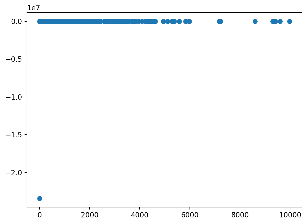
Here the pattern of minutes and consumption is not so marked as in the normal strom.

from matplotlib import pyplot
pyplot.scatter(
    waermestrom.query("minutes < 10000")["minutes"], 
    waermestrom.query("minutes < 10000")["consumption_day_equivalent"]
)

import plotly.express as px
fig = px.scatter(
    data_frame=waermestrom.query("minutes < 10000"), 
    x="minutes", 
    y="consumption_day_equivalent", hover_data=['date'],
    marginal_x="histogram", 
    marginal_y="histogram"
)
fig.show()

Consumption by hour

So, again let’s take the inefficient but straightforward way. First expand in minutes to the whole range.

%%sql

CREATE OR REPLACE TABLE waermestrom_minute_nulls AS
WITH minutes_table AS (
  SELECT UNNEST(generate_series(ts[1], ts[2], interval 1 minute)) as minute
  FROM (VALUES (
    [(SELECT MIN(date) FROM waermestrom), (SELECT MAX(DATE) FROM waermestrom)]
  )) t(ts)
)
SELECT * 
FROM minutes_table
LEFT JOIN waermestrom
ON minutes_table.minute = waermestrom.date
;
SELECT * FROM waermestrom_minute_nulls ORDER BY minute LIMIT 10;

	minute	date	value	value_hoch	value_niedrig	minutes	consumption	cm	consumption_day_equivalent	consumption_hoch	consumption_niedrig	cm_hoch	cm_niedrig
0	2016-07-04 07:50:00	2016-07-04 07:50:00	0	0	0	1440	11	0.007639	11.0	11	11	0.007639	0.007639
1	2016-07-04 07:51:00	NaT	<NA>	<NA>	<NA>	<NA>	<NA>	NaN	NaN	<NA>	<NA>	NaN	NaN
2	2016-07-04 07:52:00	NaT	<NA>	<NA>	<NA>	<NA>	<NA>	NaN	NaN	<NA>	<NA>	NaN	NaN
3	2016-07-04 07:53:00	NaT	<NA>	<NA>	<NA>	<NA>	<NA>	NaN	NaN	<NA>	<NA>	NaN	NaN
4	2016-07-04 07:54:00	NaT	<NA>	<NA>	<NA>	<NA>	<NA>	NaN	NaN	<NA>	<NA>	NaN	NaN
5	2016-07-04 07:55:00	NaT	<NA>	<NA>	<NA>	<NA>	<NA>	NaN	NaN	<NA>	<NA>	NaN	NaN
6	2016-07-04 07:56:00	NaT	<NA>	<NA>	<NA>	<NA>	<NA>	NaN	NaN	<NA>	<NA>	NaN	NaN
7	2016-07-04 07:57:00	NaT	<NA>	<NA>	<NA>	<NA>	<NA>	NaN	NaN	<NA>	<NA>	NaN	NaN
8	2016-07-04 07:58:00	NaT	<NA>	<NA>	<NA>	<NA>	<NA>	NaN	NaN	<NA>	<NA>	NaN	NaN
9	2016-07-04 07:59:00	NaT	<NA>	<NA>	<NA>	<NA>	<NA>	NaN	NaN	<NA>	<NA>	NaN	NaN

And fill in the NULLS

%%sql

CREATE OR REPLACE TABLE waermestrom_minute AS
SELECT
  minute,
  date,
  value,
  value_hoch,
  value_niedrig,
  minutes,
  consumption,
  FIRST_VALUE(cm IGNORE NULLS) OVER(
    ORDER BY minute ROWS BETWEEN CURRENT ROW AND UNBOUNDED FOLLOWING 
  ) AS cm,
  FIRST_VALUE(cm_hoch IGNORE NULLS) OVER(
    ORDER BY minute ROWS BETWEEN CURRENT ROW AND UNBOUNDED FOLLOWING 
  ) AS cm_hoch,
  FIRST_VALUE(cm_niedrig IGNORE NULLS) OVER(
    ORDER BY minute ROWS BETWEEN CURRENT ROW AND UNBOUNDED FOLLOWING 
  ) AS cm_niedrig
FROM waermestrom_minute_nulls t1
ORDER BY t1.minute
;
SELECT * FROM waermestrom_minute ORDER BY minute LIMIT 100;

	minute	date	value	value_hoch	value_niedrig	minutes	consumption	cm	cm_hoch	cm_niedrig
0	2016-07-04 07:50:00	2016-07-04 07:50:00	0	0	0	1440	11	0.007639	0.007639	0.007639
1	2016-07-04 07:51:00	NaT	<NA>	<NA>	<NA>	<NA>	<NA>	0.200000	0.100000	0.100000
2	2016-07-04 07:52:00	NaT	<NA>	<NA>	<NA>	<NA>	<NA>	0.200000	0.100000	0.100000
3	2016-07-04 07:53:00	NaT	<NA>	<NA>	<NA>	<NA>	<NA>	0.200000	0.100000	0.100000
4	2016-07-04 07:54:00	NaT	<NA>	<NA>	<NA>	<NA>	<NA>	0.200000	0.100000	0.100000
...	...	...	...	...	...	...	...	...	...	...
95	2016-07-04 09:25:00	NaT	<NA>	<NA>	<NA>	<NA>	<NA>	0.004872	0.002585	0.002287
96	2016-07-04 09:26:00	NaT	<NA>	<NA>	<NA>	<NA>	<NA>	0.004872	0.002585	0.002287
97	2016-07-04 09:27:00	NaT	<NA>	<NA>	<NA>	<NA>	<NA>	0.004872	0.002585	0.002287
98	2016-07-04 09:28:00	NaT	<NA>	<NA>	<NA>	<NA>	<NA>	0.004872	0.002585	0.002287
99	2016-07-04 09:29:00	NaT	<NA>	<NA>	<NA>	<NA>	<NA>	0.004872	0.002585	0.002287

100 rows × 10 columns

And now we can simply aggregate per day and hour, and the average will be correct, as all the rows have comparable units (consumption for one minute, with equal weight).

%%sql

consumption_hour_avg << SELECT 
  COUNT(*) AS cnt,
  hour(minute) AS hour, 
  AVG(cm)*60*24 AS cmy
FROM waermestrom_minute
GROUP BY hour(minute)
;

import plotly.express as px
fig = px.line(consumption_hour_avg, y='cmy', x='hour')
fig.show()

%%sql

consumption_hour_avg << SELECT 
  hour(minute) AS hour, 
  1.0*AVG(cm)*60*24 AS cmy
FROM waermestrom_minute
WHERE minute <= '2021-05-25' OR minute >= '2022-11-30'
GROUP BY hour(minute)
;

import plotly.express as px
fig = px.bar(consumption_hour_avg, y='cmy', x='hour')
fig.show()

Traces plot

%%sql


SELECT
  hour(minute) AS hour, 
  AVG(1.0 * 60 * 24 * cm) AS cm
FROM waermestrom_minute
WHERE minute <= '2021-05-25' OR minute >= '2022-11-30'
GROUP BY hour(minute)
;

	hour	cm
0	0	12.894955
1	1	12.836133
2	2	12.819185
3	3	12.815426
4	4	12.797544
5	5	12.771900
6	6	12.720561
7	7	12.701939
8	8	12.569834
9	9	-246.355914
10	10	12.368265
11	11	12.270323
12	12	12.155339
13	13	12.113588
14	14	12.108235
15	15	12.063699
16	16	12.024798
17	17	11.969528
18	18	12.027910
19	19	12.259541
20	20	12.714311
21	21	13.019616
22	22	13.090068
23	23	13.026564

%%sql

SELECT 
  minute,
  date,
  1.0 * 60 * 24 * cm AS cm,
  AVG(1.0 * 60 * 24 * cm) OVER(
    ORDER BY minute ROWS BETWEEN 240 PRECEDING AND CURRENT ROW
  ) AS cmma
FROM waermestrom_minute
WHERE minute > '2022-11-30'
;

	minute	date	cm	cmma
0	2022-11-30 00:01:00	NaT	11.974301	11.974301
1	2022-11-30 00:02:00	NaT	11.974301	11.974301
2	2022-11-30 00:03:00	NaT	11.974301	11.974301
3	2022-11-30 00:04:00	NaT	11.974301	11.974301
4	2022-11-30 00:05:00	NaT	11.974301	11.974301
...	...	...	...	...
1770307	2026-04-12 09:08:00	NaT	10.105263	10.105263
1770308	2026-04-12 09:09:00	NaT	10.105263	10.105263
1770309	2026-04-12 09:10:00	NaT	10.105263	10.105263
1770310	2026-04-12 09:11:00	NaT	10.105263	10.105263
1770311	2026-04-12 09:12:00	2026-04-12 09:12:00	10.105263	10.105263

1770312 rows × 4 columns

%%sql

CREATE OR REPLACE TABLE toy AS
WITH hourly_average AS (
  SELECT
    hour(minute) AS hour, 
    AVG(1.0 * 60 * 24 * cm) AS cmha
  FROM waermestrom_minute
  --This was originally here, because we wanted to see the hourly variation
  --and keeping this long period without measurements just smoothed things
  --but for waermestrom, it has a misleading implication: since we have 
  --measurements mostly in the wintertime, the average without this period
  --is high, reflecting the higher energy consumption during winter
  --WHERE minute <= '2021-05-25' OR minute >= '2022-11-30'
  GROUP BY hour(minute)
),
last_measurements AS (
  SELECT 
    minute,
    date,
    1.0 * 60 * 24 * cm AS cm,
    AVG(1.0 * 60 * 24 * cm) OVER(
      ORDER BY minute ROWS BETWEEN 60*4 PRECEDING AND CURRENT ROW
    ) AS cmma
  FROM waermestrom_minute
  WHERE minute >= '2022-11-30'
)
SELECT *, CASE WHEN date IS NOT NULL THEN cm ELSE NULL END AS cmdate
FROM last_measurements
LEFT JOIN hourly_average
ON hour(last_measurements.minute) = hourly_average.hour
;

	Success

%sql toy << SELECT * FROM toy;

import plotly.graph_objects as go
fig = px.area(toy, x='minute', y='cmha')
fig.add_trace(go.Scatter(
  x=toy['minute'], y=toy['cmma'], mode='lines', showlegend=False
))
fig.add_trace(go.Scatter(
  x=toy['date'], y=toy['cmdate'], mode='markers', showlegend=False
))

# Add range slider
fig.update_layout(
    xaxis=dict(
        rangeselector=dict(
            buttons=list([
                dict(count=1,
                     label="1m",
                     step="month",
                     stepmode="backward"),
                dict(count=7,
                     label="7d",
                     step="day",
                     stepmode="backward"),
                dict(count=15,
                     label="15d",
                     step="day",
                     stepmode="backward"),
                dict(step="all")
            ])
        ),
        rangeslider=dict(
            visible=True
        ),
        type="date"
    )
)

fig.show()

TODO: fix the range, which range?

Let’s see the rate hoch tarif vs. niedrig

niedrig_fraction << SELECT date AS day, AVG(cm_niedrig/cm) AS niedrig_fraction, AVG(cm_niedrig)/AVG(cm) AS niedrig_fraction2, AVG(niedrig_fraction) OVER( ORDER BY minute ROWS BETWEEN 60 * 24 * 7 PRECEDING AND CURRENT ROW ) AS niedrig_fraction_ma FROM waermestrom_minute GROUP BY date ORDER BY date ;

import plotly.express as px fig = px.bar(niedrig_fraction, x=‘day’, y=‘niedrig_fraction2’) fig.show()