Baseline Model

From the first look at the correlations, a model with polynomials looked fitting. So let’s here fit such a model, that would be the model to beat later down the line.

Polynomial Model

Here we stick to a simple OLS, but using a polynomial specification for the predictors temperature and air humidity, thereby, addressing one of the TODOs listed after the naive model

⏩ stepit 'baseline': Starting execution of `strom.modelling.assess_model()` 2026-04-12 13:37:22

⏩ stepit 'get_single_split_metrics': Starting execution of `strom.modelling.get_single_split_metrics()` 2026-04-12 13:37:22

✅ stepit 'get_single_split_metrics': Successfully completed and cached [exec time 0.0 seconds, cache time 0.0 seconds, size 1.0 KB] `strom.modelling.get_single_split_metrics()` 2026-04-12 13:37:22

⏩ stepit 'cross_validate_pipe': Starting execution of `strom.modelling.cross_validate_pipe()` 2026-04-12 13:37:22

[Parallel(n_jobs=-1)]: Using backend LokyBackend with 4 concurrent workers.

[Parallel(n_jobs=-1)]: Done   5 out of   5 | elapsed:    2.1s finished

✅ stepit 'cross_validate_pipe': Successfully completed and cached [exec time 2.1 seconds, cache time 0.0 seconds, size 2.2 KB] `strom.modelling.cross_validate_pipe()` 2026-04-12 13:37:24

✅ stepit 'baseline': Successfully completed and cached [exec time 2.2 seconds, cache time 0.0 seconds, size 16.0 KB] `strom.modelling.assess_model()` 2026-04-12 13:37:24

Metrics

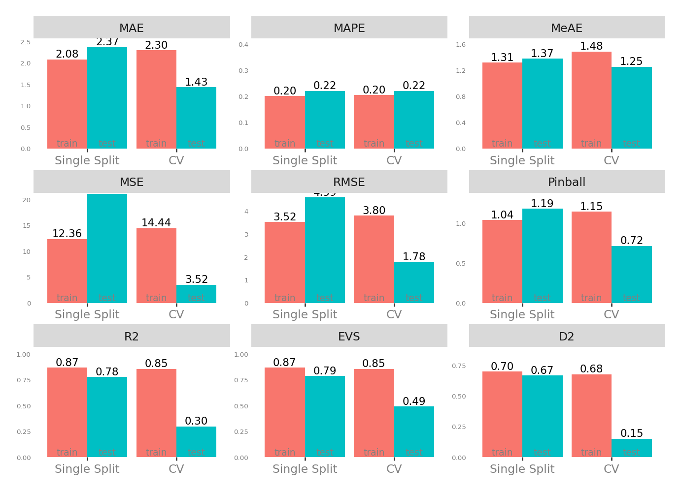
	Single Split		CV
	train	test	test	train
MAE - Mean Absolute Error	2.081643	2.474265	1.434205	2.296273
MSE - Mean Squared Error	12.356684	19.408106	3.516287	14.429139
RMSE - Root Mean Squared Error	3.515208	4.405463	1.776508	3.796345
R2 - Coefficient of Determination	0.867416	0.801708	0.296421	0.854208
MAPE - Mean Absolute Percentage Error	0.200508	0.202882	0.220062	0.204431
EVS - Explained Variance Score	0.867416	0.802337	0.490443	0.854208
MeAE - Median Absolute Error	1.314457	1.477188	1.249098	1.484622
D2 - D2 Absolute Error Score	0.699481	0.677488	0.149788	0.676571
Pinball - Mean Pinball Loss	1.040821	1.237133	0.717103	1.148137

Scatter plot matrix

Observed vs. Predicted and Residuals vs. Predicted

Check for …

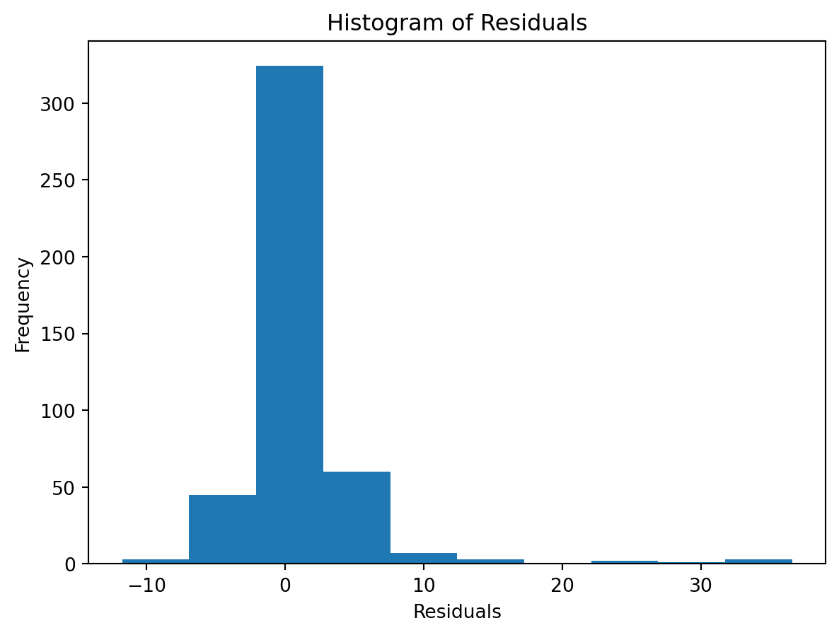
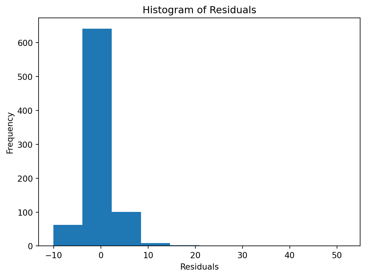
check the residuals to assess the goodness of fit.

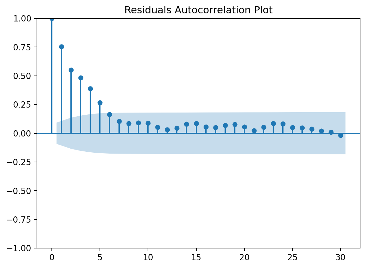
white noise or is there a pattern?
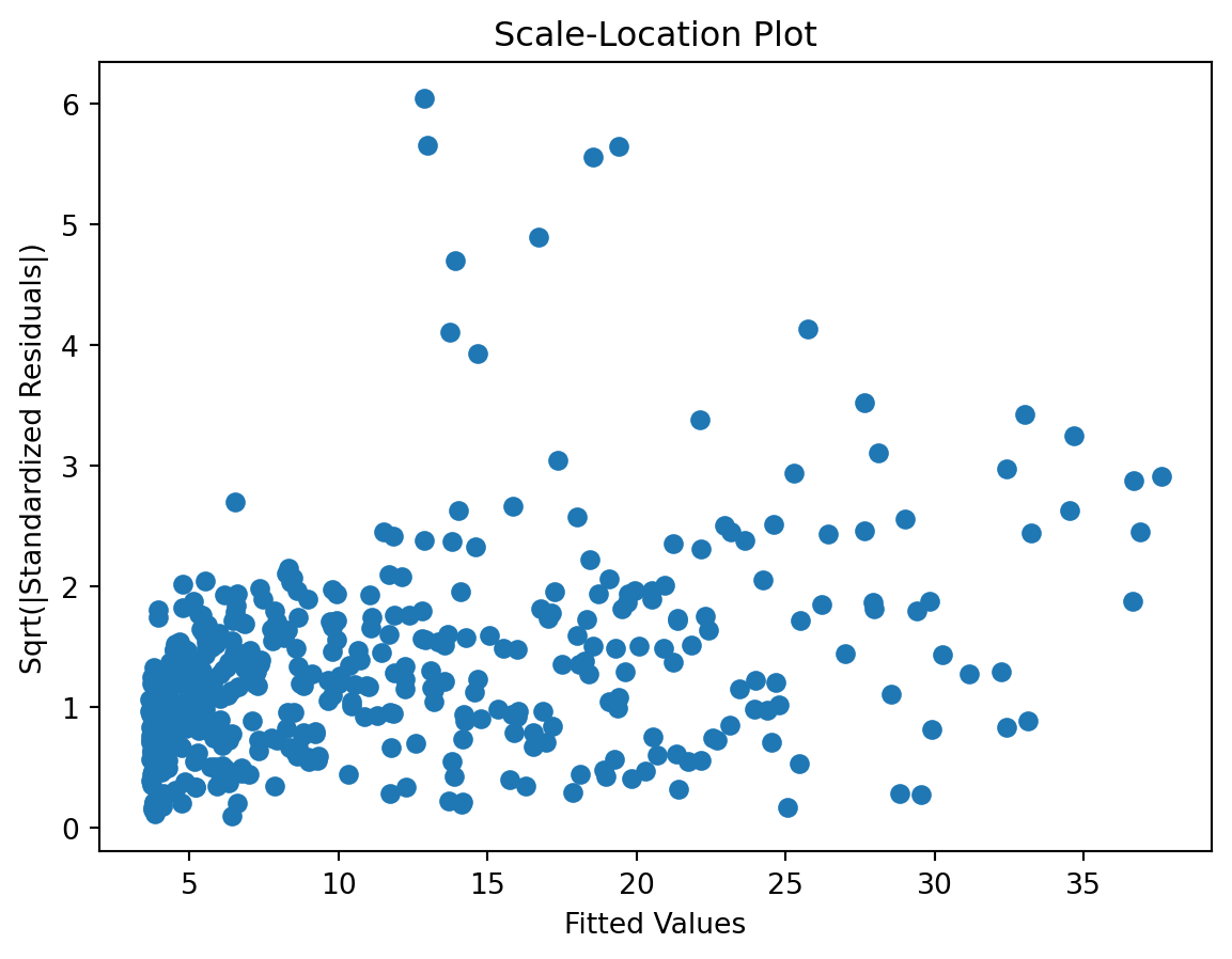
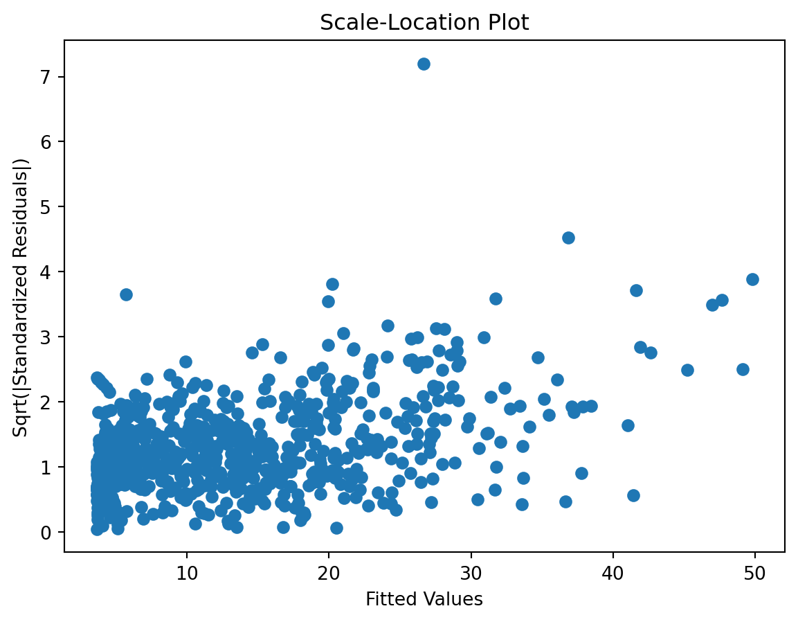
heteroscedasticity?
non-linearity?

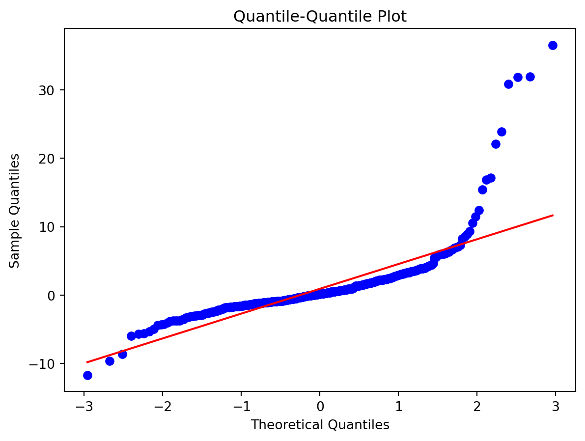
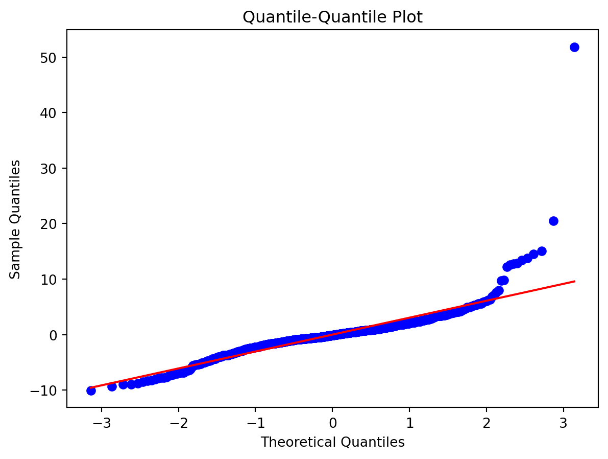
Normality of Residuals:

Check for …

Are residuals normally distributed?

Leverage

Scale-Location plot

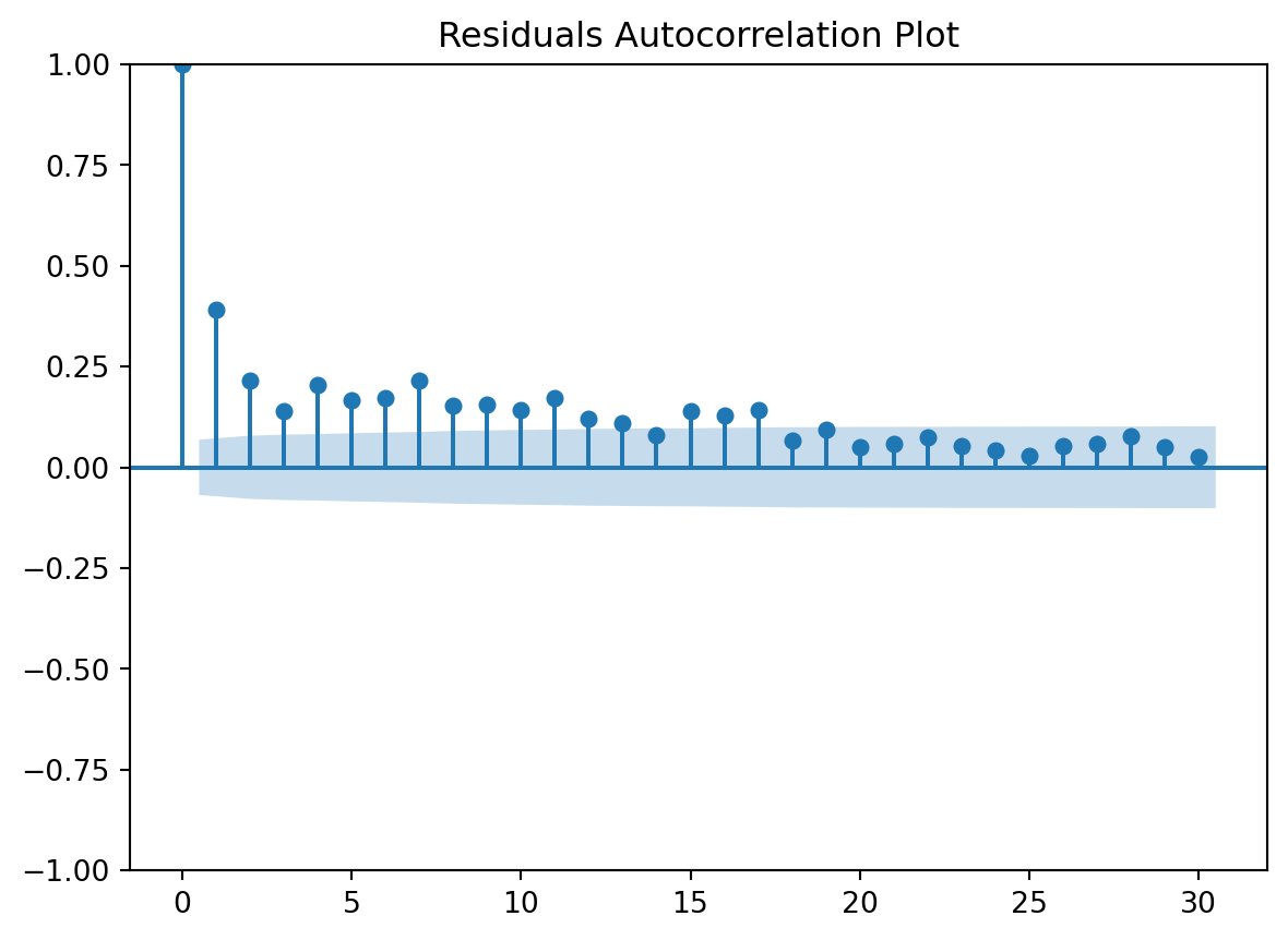
Residuals Autocorrelation Plot

Residuals vs Time

TODOs

Substantial improvement here, we still have some items in the to-do list and given these results, I would add a coulpe more:

Check the degree of the polynomial
depite the much better fit, there are still some -although minor- heteroscedaticity, mostly associated to the lowest temperatures where the variance of strom use is higher. Here we can try other models that better handle that long tail, and also, try transformations.
there might be also a seasonal pattern, because we are not accounting for, for example, weekends and so on. Here we can see if the seasonal trend decomposition can help.
finally, there is still some evidence of autocorrelation. Which kinda makes sense: it is not the same to have one day with a very low temperature compared to a whole week with very low temperatures: while the former could be wintered with the heat already produced, as long as there is not much energy lose, the latter would certainly need much more work from the wärmepumpe to keep fighting the cold. In that sense, it seems unrealistic to just assume that the increase energy consumption of several days of extreme cold is just the sum of the daily increases. So if the one-day-increase due to extreme cold is 10, five consecutve days would probably result in an increase greater than 10*5=50, probably much greater. But let’s explore such hipothesis in the data and try to accomodate that in the model using lags, or moving average of the last few days.
run some PCA, with min, max mean and so on and think about a Cumulative Explained Variance plot https://archive.is/X1wrZ#selection-1059.8-1059.37 PCA seems sensible, because several climatic variables are highly correlated, but still could have different signals. E.g. temperature, the mean seems to capture well the process, but beyond that, how much it varies min, max, std dev, seems to have some predictive power.
perhaps experiment with feature selection.
and consider log-transforming the target, after all, the distribution of it is right-skewed with relatively long right tail
Consider models to handle censored data, since the consumption can never be negative. This, being a linear model, can still predict negative values, even though the polynomial show a rather good fit. But there is no restriction and in fact, in the test set, in the warm period with low consumption, there are a few instances in which the model ends up predicting negative values. So we would need to take that into account and add some sort of constraint for that.
Handle the outliers. These are really just a couple of points, but at least in these kind of model, they end up having a high leverage. So, we could just handle them by replacing them with locally-defined averages, or use models that are robust to those.

Polynomials but using statsmodels …

                            OLS Regression Results                            
==============================================================================
Dep. Variable:                     wd   R-squared:                       0.848
Model:                            OLS   Adj. R-squared:                  0.847
Method:                 Least Squares   F-statistic:                     707.4
Date:                Sun, 12 Apr 2026   Prob (F-statistic):               0.00
Time:                        13:37:28   Log-Likelihood:                -3861.4
No. Observations:                1402   AIC:                             7747.
Df Residuals:                    1390   BIC:                             7810.
Df Model:                          11                                         
Covariance Type:            nonrobust                                         
=======================================================================================
                          coef    std err          t      P>|t|      [0.025      0.975]
---------------------------------------------------------------------------------------
Intercept              27.2336      2.654     10.261      0.000      22.027      32.440
tt_tu_mean             -1.9909      0.083    -24.046      0.000      -2.153      -1.828
I(tt_tu_mean ** 2)      0.0937      0.008     11.849      0.000       0.078       0.109
I(tt_tu_mean ** 3)     -0.0013      0.001     -1.291      0.197      -0.003       0.001
I(tt_tu_mean ** 4)  -7.429e-05   8.62e-05     -0.862      0.389      -0.000    9.47e-05
I(tt_tu_mean ** 5)   2.696e-06   2.11e-06      1.278      0.201   -1.44e-06    6.83e-06
rf_tu_mean              0.0370      0.033      1.116      0.265      -0.028       0.102
rf_tu_min              -0.0328      0.017     -1.939      0.053      -0.066       0.000
rf_tu_max              -0.0469      0.039     -1.199      0.231      -0.124       0.030
tt_tu_mean.shift(1)    -0.2229      0.073     -3.066      0.002      -0.366      -0.080
tt_tu_mean.shift(2)     0.0442      0.071      0.620      0.535      -0.096       0.184
tt_tu_mean.shift(3)    -0.0663      0.049     -1.367      0.172      -0.161       0.029
==============================================================================
Omnibus:                     1359.610   Durbin-Watson:                   0.837
Prob(Omnibus):                  0.000   Jarque-Bera (JB):           111116.297
Skew:                           4.328   Prob(JB):                         0.00
Kurtosis:                      45.746   Cond. No.                     4.65e+07
==============================================================================

Notes:
[1] Standard Errors assume that the covariance matrix of the errors is correctly specified.
[2] The condition number is large, 4.65e+07. This might indicate that there are
strong multicollinearity or other numerical problems.

Model Cards provide a framework for transparent, responsible reporting. 
 Use the vetiver `.qmd` Quarto template as a place to start, 
 with vetiver.model_card()
Writing pin:
Name: 'waermestrom'
Version: 20260412T133728Z-089b0

<vetiver.vetiver_model.VetiverModel at 0x7ff318feb640>

here’s also the polynomial model, but using scikit-learn

0.8477166938392322