Let’s address here a couple of the to-dos from the previous pages. Namely, let’s check the degree of the polynomial using a grid search and checkout other climatic variables, playing a bit with variable selection.
Tune polynomial degree
First, let’s fine-tune the degree of the polynomial. From the initial scatter plots, it seems that a 2 or 3 degree polynomial would be good. But let’s throw a grid search on that.
⏩ stepit 'grid_search_pipe': Starting execution of `strom.modelling.grid_search_pipe()` 2026-04-12 13:37:40✅ stepit 'grid_search_pipe': Successfully completed and cached [exec time 2.3 seconds, cache time 0.0 seconds, size 19.4 KB] `strom.modelling.grid_search_pipe()` 2026-04-12 13:37:43
It seems degree 4 would be best. Of course there is a a small variation according to the metric/scorer used, but overall, I think 4 seems best. The differences are rather small, but there is still this tension between MAE and RSME. A model that better fit on the warmer season and therefore has smaller small errors and a small MAE, tend to have a few very large errors, affecting the RSME. And the other way around.
Variable selection
Now let’s try here a brute-force approach to variable selection. Thereby, taking a not-so-thoughtful-but-quick-and-effective approach to trying out other climatic variables and checking the associations with relative humidity and other variables, to see if there is indeed a signal or just noise in some of them like humidity and so on.
Just let it crunch through a bunch of variable combinations. There will be many non-sensical or irrelevant combinations. But it’s just fast to write and the machine will have to work, me not so much.
From topic knowledge and the first correlations observed, we would expect mostly temprature to play a key role in the model. Yet, other variables such a humidity, pressure or condensation point could also be relevant. So let’s throw all that into a grid search and see what it spits out of it.
tt: Temperatur der Luft in 2m Hoehe °C
rf_tu: relative Feuchte %
td: Taupunktstemperatur °C
vp_std: berechnete Stundenwerte des Dampfdruckes hpa
tf_std: berechnete Stundenwerte der Feuchttemperatur °C
p_std: Stundenwerte Luftdruck hpa
⏩ stepit 'grid_search_pipe': Starting execution of `strom.modelling.grid_search_pipe()` 2026-04-12 13:37:43✅ stepit 'grid_search_pipe': Successfully completed and cached [exec time 1.0 seconds, cache time 0.0 seconds, size 46.1 KB] `strom.modelling.grid_search_pipe()` 2026-04-12 13:37:44
Loading ITables v2.5.2 from the init_notebook_mode cell...
(need help?)
Well humidity and other climatic variables can only improve the model marginally. A proper mediation analysis would still be in order, but this at least shed some light on it. Interestingly, some models without temperature but the set of other climatic variables almost equal the performance of the best model with temperature. Overall, it seems that at least temperature, humidity and pressure should be considered. Yet, the tend to be collineal and thus not really be able to used them all just like that in this kind of model.
One last brute-force approach for today and let automatically choose the best model
In a Jupyter environment, please rerun this cell to show the HTML representation or trust the notebook. On GitHub, the HTML representation is unable to render, please try loading this page with nbviewer.org.
Parameters
steps
[('vars', ...), ('polynomial', ...), ...]
transform_input
None
memory
None
verbose
False
Parameters
columns
['tf_std_mean']
Parameters
degree
5
interaction_only
False
include_bias
True
order
'C'
Parameters
fit_intercept
True
copy_X
True
tol
1e-06
n_jobs
None
positive
False
Loading ITables v2.5.2 from the init_notebook_mode cell...
(need help?)
Loading ITables v2.5.2 from the init_notebook_mode cell...
(need help?)
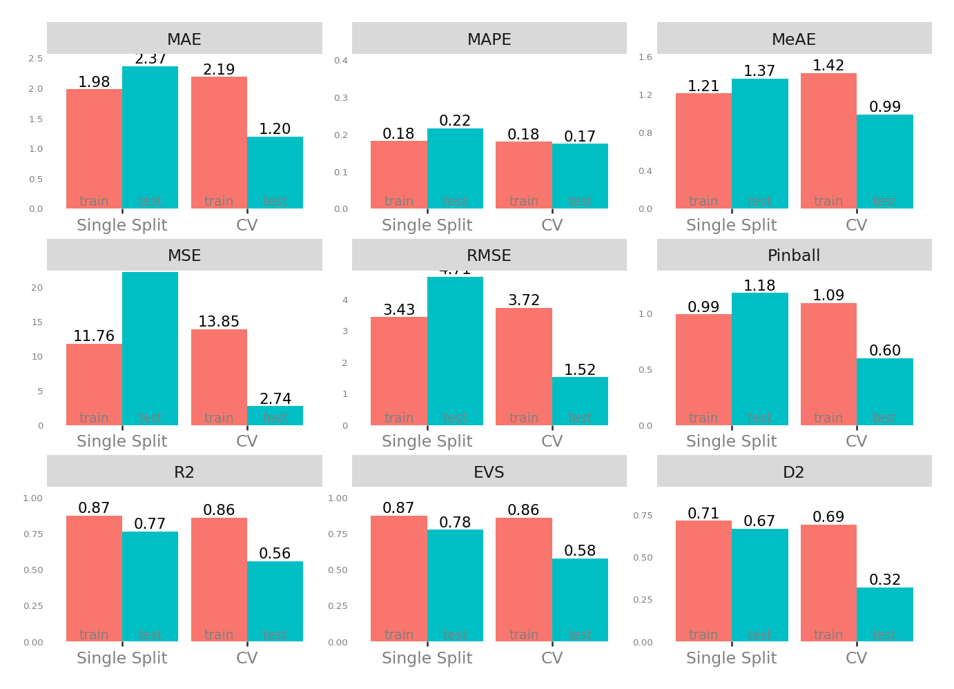
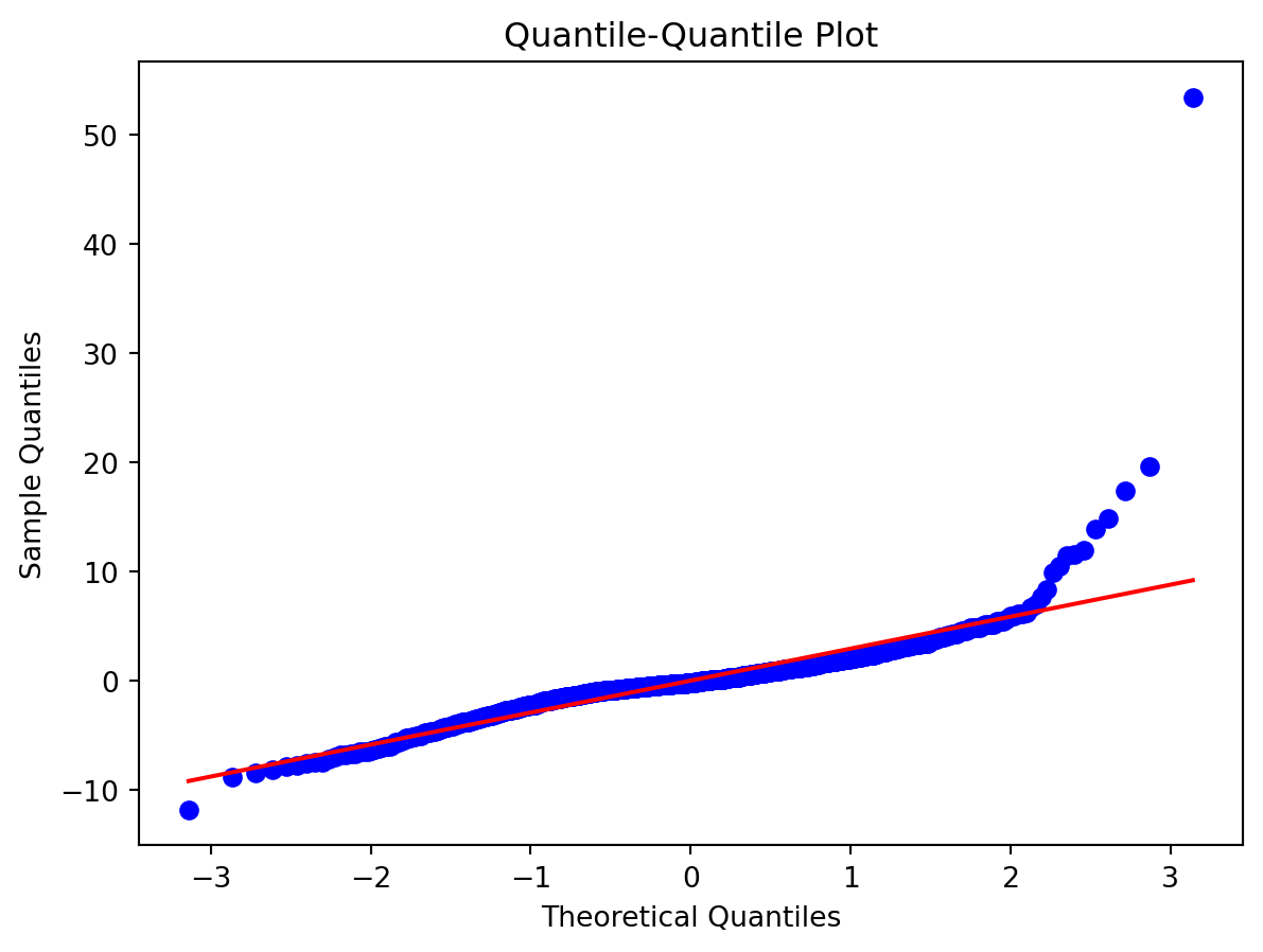
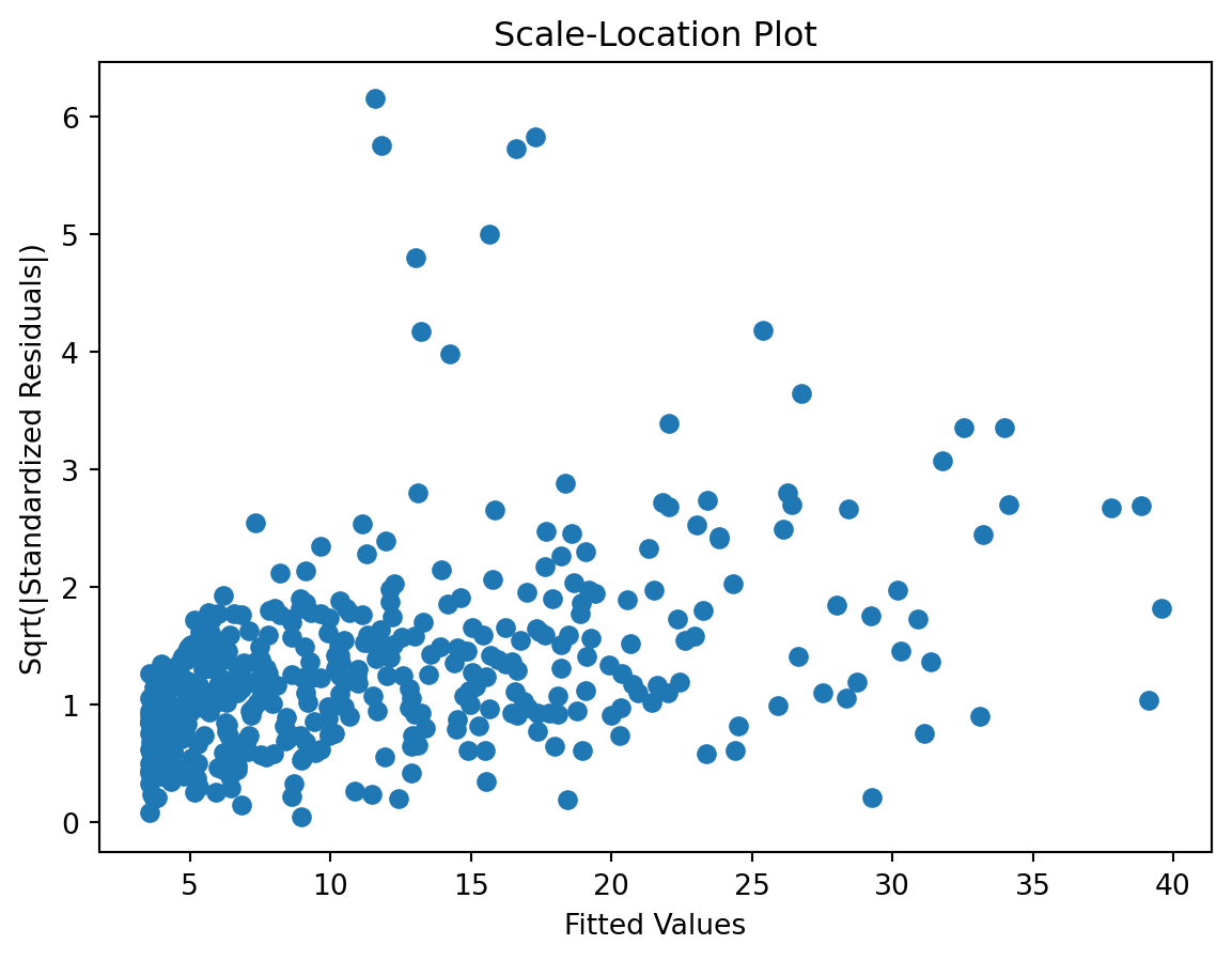
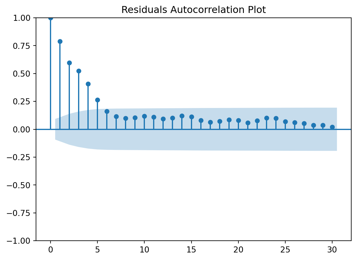
Assessment of the best model in that brute force approach
⏩ stepit 'poly': Starting execution of `strom.modelling.assess_model()` 2026-04-12 13:37:48⏩ stepit 'get_single_split_metrics': Starting execution of `strom.modelling.get_single_split_metrics()` 2026-04-12 13:37:48✅ stepit 'get_single_split_metrics': Successfully completed and cached [exec time 0.0 seconds, cache time 0.0 seconds, size 1.0 KB] `strom.modelling.get_single_split_metrics()` 2026-04-12 13:37:48⏩ stepit 'cross_validate_pipe': Starting execution of `strom.modelling.cross_validate_pipe()` 2026-04-12 13:37:48
[Parallel(n_jobs=-1)]: Using backend LokyBackend with 4 concurrent workers.
[Parallel(n_jobs=-1)]: Done 5 out of 5 | elapsed: 0.0s finished
✅ stepit 'cross_validate_pipe': Successfully completed and cached [exec time 0.0 seconds, cache time 0.0 seconds, size 2.2 KB] `strom.modelling.cross_validate_pipe()` 2026-04-12 13:37:48✅ stepit 'poly': Successfully completed and cached [exec time 0.1 seconds, cache time 0.0 seconds, size 16.0 KB] `strom.modelling.assess_model()` 2026-04-12 13:37:48
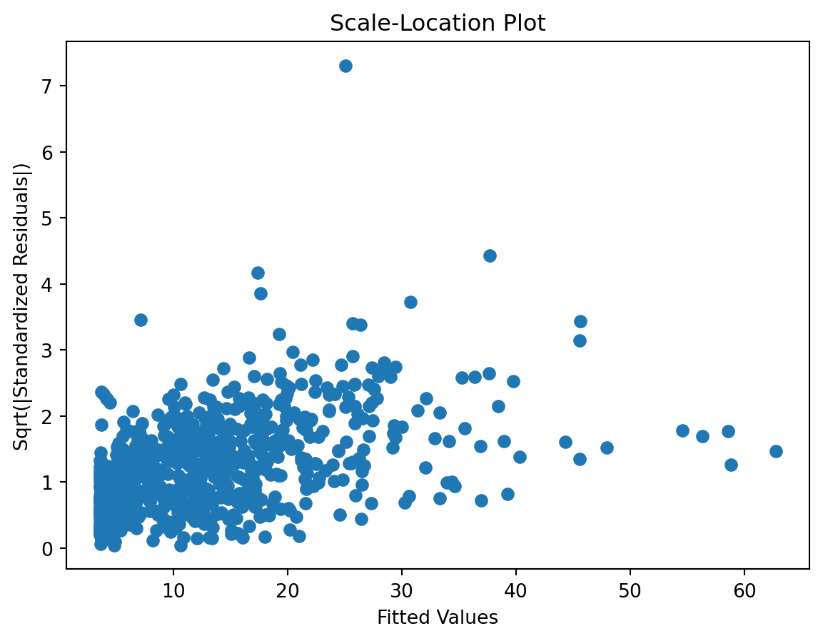
So let’s compare the models with and without humidity.
Cross-validation messages
♻️ stepit 'cross_validate_pipe': is up-to-date. Using cached result for `strom.modelling.cross_validate_pipe()` 2026-04-12 13:37:52⏩ stepit 'cross_validate_pipe': Starting execution of `strom.modelling.cross_validate_pipe()` 2026-04-12 13:37:52
[Parallel(n_jobs=-1)]: Using backend LokyBackend with 4 concurrent workers.
[Parallel(n_jobs=-1)]: Done 5 out of 5 | elapsed: 0.1s finished
✅ stepit 'cross_validate_pipe': Successfully completed and cached [exec time 0.1 seconds, cache time 0.0 seconds, size 2.2 KB] `strom.modelling.cross_validate_pipe()` 2026-04-12 13:37:52♻️ stepit 'cross_validate_pipe': is up-to-date. Using cached result for `strom.modelling.cross_validate_pipe()` 2026-04-12 13:37:52
In a Jupyter environment, please rerun this cell to show the HTML representation or trust the notebook. On GitHub, the HTML representation is unable to render, please try loading this page with nbviewer.org.
In a Jupyter environment, please rerun this cell to show the HTML representation or trust the notebook. On GitHub, the HTML representation is unable to render, please try loading this page with nbviewer.org.
In a Jupyter environment, please rerun this cell to show the HTML representation or trust the notebook. On GitHub, the HTML representation is unable to render, please try loading this page with nbviewer.org.
Parameters
steps
[('vars', ...), ('polynomial', ...), ...]
transform_input
None
memory
None
verbose
False
Parameters
columns
['tf_std_mean']
Parameters
degree
5
interaction_only
False
include_bias
True
order
'C'
Parameters
fit_intercept
True
copy_X
True
tol
1e-06
n_jobs
None
positive
False
A nice improvement over the baseline model, and the model without humidity is slightly better across all metrics (a rather small improvement, but across all metrics).